R言語のggplotにおいて、グラフに回帰直線の式を表示する方法をお伝えします。
ggplotのグラフに回帰直線の式を表示する方法はいくつかあります。ここでは最も簡単と思われるggpmiscパッケージを用いて回帰直線の式を表示する方法をお伝えします。
環境
今回の作業環境をsessionInfo()関数で確認しておきます。
sessionInfo()

R version 4.0.2 (2020-06-22)
Platform: x86_64-pc-linux-gnu (64-bit)
Running under: Ubuntu 20.04.1 LTS

Matrix products: default
BLAS:   /usr/lib/x86_64-linux-gnu/blas/libblas.so.3.9.0
LAPACK: /usr/lib/x86_64-linux-gnu/lapack/liblapack.so.3.9.0

locale:
 [1] LC_CTYPE=ja_JP.UTF-8       LC_NUMERIC=C               LC_TIME=ja_JP.UTF-8        LC_COLLATE=ja_JP.UTF-8
 [5] LC_MONETARY=ja_JP.UTF-8    LC_MESSAGES=ja_JP.UTF-8    LC_PAPER=ja_JP.UTF-8       LC_NAME=C
 [9] LC_ADDRESS=C               LC_TELEPHONE=C             LC_MEASUREMENT=ja_JP.UTF-8 LC_IDENTIFICATION=C

attached base packages:
[1] stats     graphics  grDevices utils     datasets  methods   base

other attached packages:
 [1] ggpmisc_0.3.6   forcats_0.5.0   stringr_1.4.0   dplyr_1.0.2     purrr_0.3.4     readr_1.3.1     tidyr_1.1.2     tibble_3.0.3
 [9] ggplot2_3.3.2   tidyverse_1.3.0
準備
あらかじめtidyverseパッケージとggpmiscパッケージを読み込んでおきます。また、Rに標準で組み込まれているOrangeをサンプルデータとして用いることにします。
library(tidyverse)
library(ggpmisc)

data("Orange")

df <- Orange %>%
  filter(Tree %in% c("1"))
ggpmiscパッケージを用いて回帰直線の式を表示
ggpmiscパッケージは、ggplotのグラフに回帰直線の式や決定係数などを表示する機能を提供しています。この機能はstat_poly_eq()を通して表示することができます。回帰直線に関する表示項目は次になります。
| 指定 | 意味 |
|---|---|
| eq.label | 近似多項式の方程式 |
| rr.label | 近似モデルの決定係数 |
| adj.rr.label | 近似モデルの調整済み決定係数R^2 |
| f.value.label | 近似モデル全体のF値と自由度 |
| p.value.label | 上記のF値のP値 |
| AIC.label | 近似モデルのAIC |
| BIC.label | 近似モデルのBIC |
これらの指定は、stat()関数の引数で設定し、stat_poly_eq()関数の引数に「parse = TRUE」を設定します。具体例は以下をご参照ください。
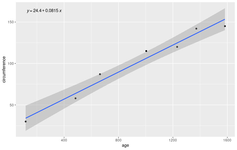
回帰直線の式を表示
g <- ggplot(df, aes(x = age, y = circumference))
g <- g + geom_point()
g <- g + geom_smooth(method = "lm", formula = y ~ x)
g <- g + stat_poly_eq(formula = y ~ x,
                      aes(label = paste(stat(eq.label))),
                      parse = TRUE)
plot(g)
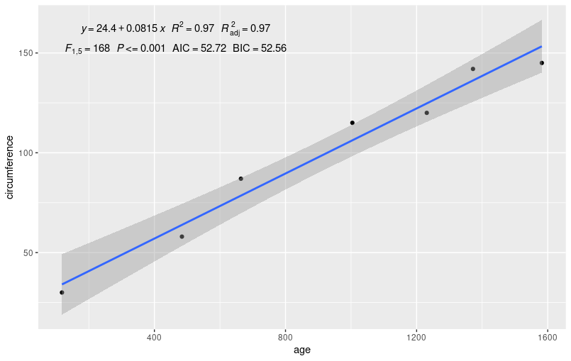
すべてのラベルを表示
g <- ggplot(df, aes(x = age, y = circumference))
g <- g + geom_point()
g <- g + geom_smooth(method = "lm", formula = y ~ x)
g <- g + stat_poly_eq(formula = y ~ x,
                      aes(label = paste(stat(eq.label),
                                        stat(rr.label),
                                        stat(adj.rr.label),
                                        stat(f.value.label),
                                        stat(p.value.label),
                                        stat(AIC.label),
                                        stat(BIC.label),
                                        sep = "~~~")),
                      parse = TRUE)
plot(g)

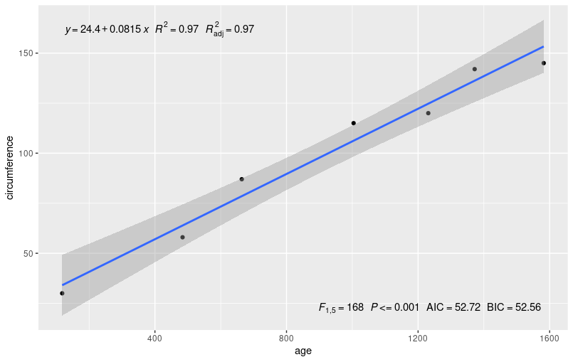
左上と右下にラベルを表示
g <- ggplot(df, aes(x = age, y = circumference))
g <- g + geom_point()
g <- g + geom_smooth(method = "lm", formula = y ~ x)
g <- g + stat_poly_eq(formula = y ~ x,
                      aes(label = paste(stat(eq.label),
                                        stat(rr.label),
                                        stat(adj.rr.label),
                                        sep = "~~~")),
                      parse = TRUE)
g <- g + stat_poly_eq(formula = y ~ x,
                      aes(label = paste(stat(f.value.label),
                                        stat(p.value.label),
                                        stat(AIC.label),
                                        stat(BIC.label),
                                        sep = "~~~")),
                      label.x = "right",
                      label.y = "bottom",
                      parse = TRUE)
plot(g)
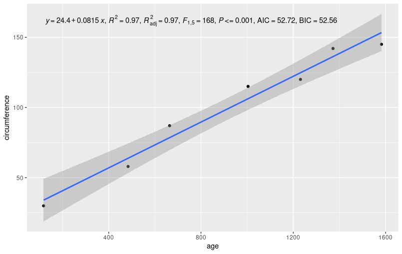
ラベルの区切り文字をスペース( )からカンマ(,)に変更
g <- ggplot(df, aes(x = age, y = circumference))
g <- g + geom_point()
g <- g + geom_smooth(method = "lm", formula = y ~ x)
g <- g + stat_poly_eq(formula = y ~ x,
                      aes(label = paste(stat(eq.label),
                                        stat(rr.label),
                                        stat(adj.rr.label),
                                        stat(f.value.label),
                                        stat(p.value.label),
                                        stat(AIC.label),
                                        stat(BIC.label),
                                        sep = "*\", \"*")),
                      parse = TRUE)
plot(g)
ラベルを2行に分けて表示
g <- ggplot(df, aes(x = age, y = circumference))
g <- g + geom_point()
g <- g + geom_smooth(method = "lm", formula = y ~ x)
g <- g + stat_poly_eq(formula = y ~ x,
                      aes(label = paste("atop(",
                                        paste(stat(eq.label),
                                              stat(rr.label),
                                              stat(adj.rr.label),
                                              sep = "~~~"),
                                        ",",
                                        paste(stat(f.value.label),
                                              stat(p.value.label),
                                              stat(AIC.label),
                                              stat(BIC.label),
                                              sep = "~~~"),
                                        ")",
                                        sep = "")),
                      parse = TRUE)
plot(g)
yからyハットにxをzに変更して表示
g <- ggplot(df, aes(x = age, y = circumference))
g <- g + geom_point()
g <- g + geom_smooth(method = "lm", formula = y ~ x)
g <- g + stat_poly_eq(formula = y ~ x,
                      aes(label = paste(stat(eq.label),
                                        stat(rr.label),
                                        stat(adj.rr.label),
                                        stat(f.value.label),
                                        stat(p.value.label),
                                        stat(AIC.label),
                                        stat(BIC.label),
                                        sep = "~~~")),
                      eq.with.lhs = "italic(hat(y))~`=`~",
                      eq.x.rhs = "~italic(z)",
                      parse = TRUE)
plot(g)

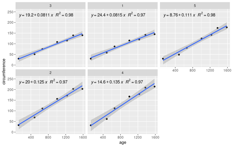
ファセットに対して適用
g <- ggplot(Orange, aes(x = age, y = circumference))
g <- g + geom_point()
g <- g + geom_smooth(method = "lm", formula = y ~ x)
g <- g + stat_poly_eq(formula = y ~ x,
                      aes(label = paste(stat(eq.label),
                                        stat(rr.label),
                                        sep = "~~~")),
                      parse = TRUE)
g <- g + facet_wrap(~ Tree)
plot(g)
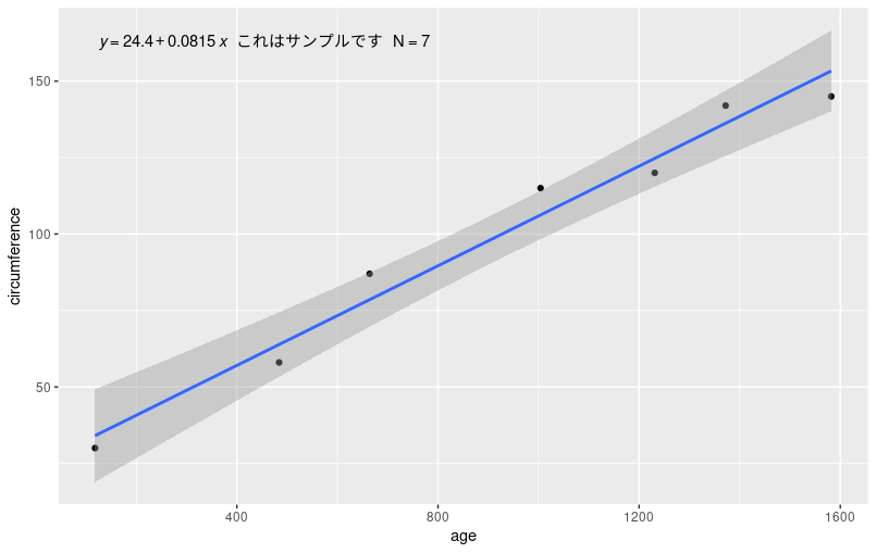
任意の文字を追加して表示
任意の文字を追加して表示する方法は次になります。注意点としては、記号「=」を表示するときは「~`=`~」に置き換えて記載します。
g <- ggplot(df, aes(x = age, y = circumference))
g <- g + geom_point()
g <- g + geom_smooth(method = "lm", formula = y ~ x)
g <- g + stat_poly_eq(formula = y ~ x,
                      aes(label = paste(stat(eq.label),
                                        paste("これはサンプルです"),
                                        paste("N ~`=`~", nrow(df)),
                                        sep = "~~~")),
                      parse = TRUE)
plot(g)